A model of ion channel gating and current
This chapter describes a generic ion channel, and provides a foundation for later chapters where specific channels of sodium and potassium are described. The theory here is the basis for the practical modelling tutorial in HH Tutorial 5.
Chemical theory and entropy
A good example of a model based on a first order equation is the one used by Hodgkin and Huxley 1 to describe the gating behaviour of an ion channel. Before we describe the gating behaviour of an ion channel, however, we need to explain the concepts of the ‘Nernst potential’ and channel conductance.
An ion channel is a protein or protein complex embedded in the bi-lipid membrane surrounding a cell and containing a pore through which an ion \(Y^{+}\) (or \(Y^{-}\)) can pass when the channel is open. If the concentration of this ion is \(\left\lbrack Y^{+} \right\rbrack_{o}\) outside the cell and \(\left\lbrack Y^{+} \right\rbrack_{i}\) inside the cell, the force driving an ion through the pore is calculated from the change in entropy.
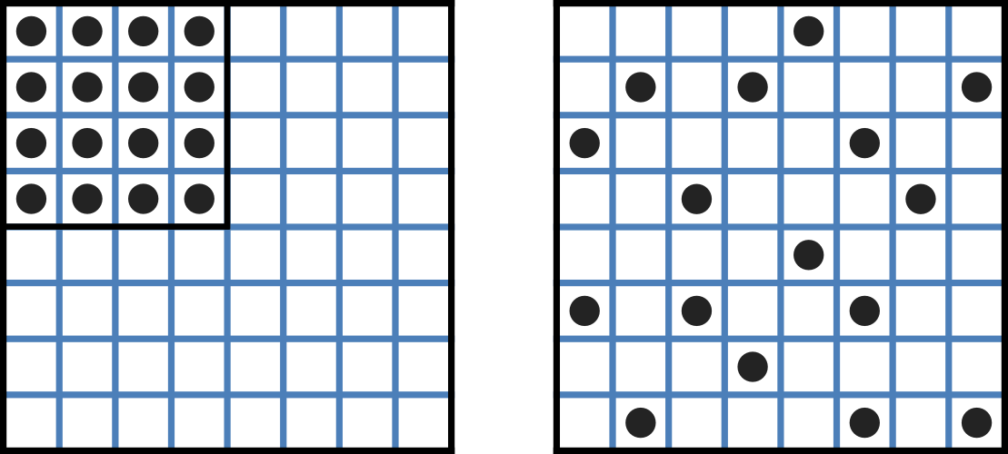
Figure 2 Distribution of microstates in a system 2. The 16 particles in a confined region (left) have only one possible arrangement (\(W=1\)) and therefore zero entropy (\(k_{B}\ln W=0\)). When the barrier is removed and the number of possible locations for each particle increases four-fold (right), the number of possible arrangements for the 16 particles increases by 416 and the increase in entropy is therefore \(\ln(416)=16\ln(4)\). The thermal energy (temperature) of the previously confined particles on the left has been redistributed in space to achieve a more probable (higher entropy) state. If we now added more particles to the container on the right, the concentration would increase and the entropy would decrease.
Entropy \(S\) in \(J.K^{-1}\) is a measure of the number of microstates available to a system, as defined by Boltzmann’s equation:
where \(W\) is the number of ways of arranging a given distribution of microstates of a system and \(k_{B}\) is Boltzmann’s constant 3. The driving force for ion movement is the dispersal of energy into a more probable distribution (see Figure: Distribution of microstates in a system 2. The 16 particles in a confined region (left) have only one possible arrangement (W=1) and therefore zero entropy (k_{B}\ln W=0). When the barrier is removed and the number of possible locations for each particle increases four-fold (right), the number of possible arrangements for the 16 particles increases by 416 and the increase in entropy is therefore \ln(416)=16\ln(4). The thermal energy (temperature) of the previously confined particles on the left has been redistributed in space to achieve a more probable (higher entropy) state. If we now added more particles to the container on the right, the concentration would increase and the entropy would decrease. ; cf. the second law of thermodynamics 4).
The energy change \(\Delta q\) associated with this change of entropy \(\Delta S\) at temperature \(T\) is \(\Delta q = T\Delta S\) in \(J\).
For a given volume of fluid the number of microstates \(W\) available to a solute (and hence the entropy of the solute) at a high concentration is less than that for a low concentration 5. The energy difference which drives ion movement from a high ion concentration \(\left\lbrack Y^{+} \right\rbrack_{i}\) (lower entropy) to a lower ion concentration \(\left\lbrack Y^{+} \right\rbrack_{o}\) (higher entropy) is therefore:
or
where
is the ‘universal gas constant’6. At 25°C (\(298K\)) \({RT} \approx 2.5 \text{ }(kJ.mol^{-1})\).
Electrical theory
Every positively charged ion that crosses the membrane raises the potential difference and produces an electrostatic driving force that opposes the entropic force (see Figure: The balance between entropic and electrostatic forces determines the Nernst potential.). To move an electron of charge \(e\) (\(\approx 1.6\times 10^{-19}\text{ }(C)\)) through a voltage change of \(\Delta\phi\) ( in \(V\)) requires energy \(e\Delta\phi\) (in \(J\)) and therefore the energy needed to move an ion \(Y^{+}\) of valence \(z=1\) (the number of charges per ion) through a voltage change of \(\Delta\phi\) is \({ze}\Delta\phi\) (\(J.ion^{-1}\)) or \({ze}N_{A}\Delta\phi\) (\(J.mol^{-1}\)). Using Faraday’s constant \(F = eN_{A}\), where \(F \approx 0.96\times10^{5}\) (\(C.mol^{-1}\)), the change in energy density at the macroscopic scale is \({zF}\Delta\phi\) (\(J.mol^{-1}\)).
No further movement of ions takes place when the force for entropy driven ion movement exactly equals the opposing electrostatic driving force associated with charge movement:
or
where \(E_{Y}\) is the “equilibrium” or “Nernst” potential for \(Y^{+}\). At 25°C (298K), \(\frac{{RT}}{F} = \frac{2.5\times10^{3}\ }{0.96\times10^{5}}\text{ }(J.C^{-1}) \approx 25mV\).
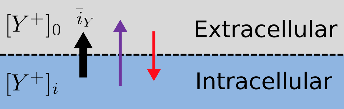
Figure 3 The balance between entropic and electrostatic forces determines the Nernst potential.
Mathematical modelling
For an open channel the electrochemical current flow is driven by the open channel conductance \({\overset{\overline{}}{g}}_{Y}\) times the difference between the transmembrane voltage \(V\) and the Nernst potential for that ion:
This defines a linear current-voltage relation (“Ohm’s law”) as shown in Figure (a) Open channel linear current-voltage relation. (b) Ion channel gating kinetics. y is the fraction of gates in the open state. \alpha_n and \beta_n are the rate constants for opening and closing, respectively. (a). The specific characteristics of a channel’s behaviour depend on how its gates modify the open channel conductance.
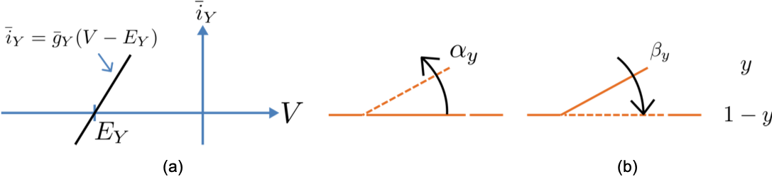
Figure 4 (a) Open channel linear current-voltage relation. (b) Ion channel gating kinetics. \(y\) is the fraction of gates in the open state. \(\alpha_n\) and \(\beta_n\) are the rate constants for opening and closing, respectively.
To describe the time dependent transition between the closed and open states of the channel, Hodgkin and Huxley introduced the idea of channel gates that control the passage of ions through a membrane ion channel. If the fraction of gates that are open is \(y\), the fraction of gates that are closed is \(1-y\), and a first order ODE can be used to describe the transition between the two states (see Figure (a) Open channel linear current-voltage relation. (b) Ion channel gating kinetics. y is the fraction of gates in the open state. \alpha_n and \beta_n are the rate constants for opening and closing, respectively. (b)).
where \(\alpha_{y}\)is the opening rate and \(\beta_{y}\) is the closing rate.
The solution to this ODE is:
The constant \(A\) can be interpreted as:
as in the previous example and, with \(y\left( 0 \right) = 0\) (i.e. all gates initially shut), the solution looks like Figure Transient behaviour for one gate (left) and γ gates in series (right). Note that the right hand graph has an initial S-shaped increase, reflecting the multiple gates in series. (a). The experimental data obtained by Hodgkin and Huxley for the squid axon indicated that the initial current flow began more slowly, as in Figure Transient behaviour for one gate (left) and γ gates in series (right). Note that the right hand graph has an initial S-shaped increase, reflecting the multiple gates in series. (b).
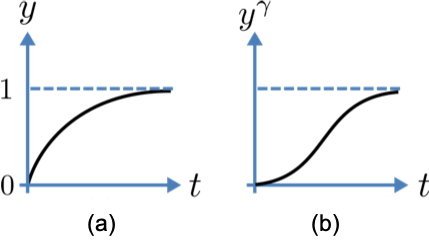
Figure 5 Transient behaviour for one gate (left) and γ gates in series (right). Note that the right hand graph has an initial S-shaped increase, reflecting the multiple gates in series.
Hodgkin and Huxley modelled this by proposing a series of gates within the ion channel. Conduction can only occur when each gate is at least partially open. Since \(y\) is the probability of a gate being open, \(y^{\gamma}\) is the probability of \(\gamma\) gates being open (since they are assumed to be independent), so the current through the channel is:
where
is the steady state current through the open gate.
Simulation and results
The formulation of a model for the generic ion channel described here is the focus of Tutorial 5. The results shown here come from that model, where parameters representing \(\gamma = 4\) gates transitioning from the closed to the open state at a membrane voltage \(V = 0\), and opening and closing rate constants of \(\alpha_{y} = 1\) ms-1 and \(\beta_{y} = 2\) ms-1.
The modelled behaviour of a single gate is shown by the green line in Figure: Dynamics of opening status for a single gate, and the resulting current for \gamma=4 gates in series., and the resulting channel current for four gates in series by the blue line. Note the slow start to the current trace in comparison with the single gate transient \(y\left( t \right)\), as observed experimentally by Hodgkin and Huxley.
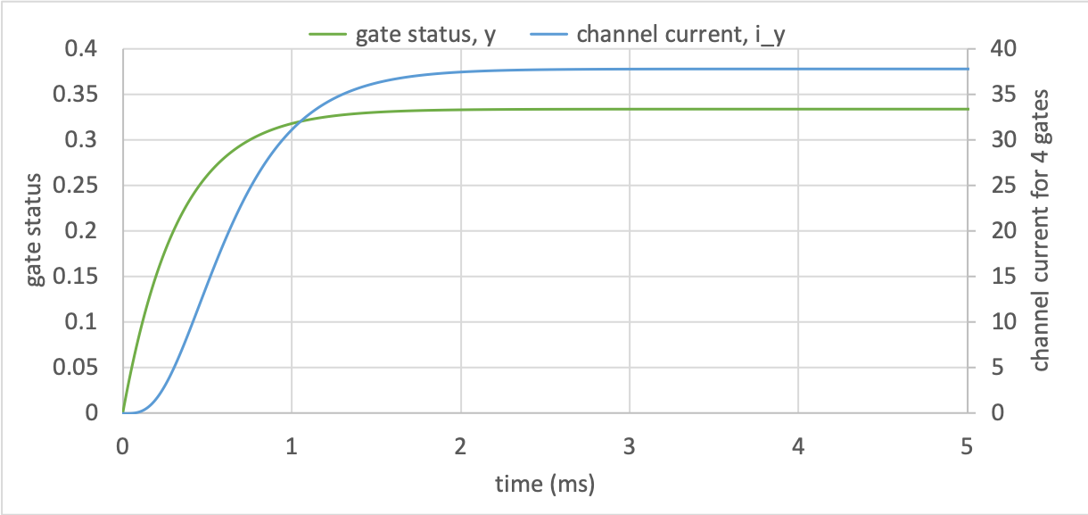
Figure 6 Dynamics of opening status for a single gate, and the resulting current for \(\gamma=4\) gates in series.
Next steps
The model of a gated ion channel presented here is used in the next two sections for the neural potassium and sodium channels. The gates create the transience of the channel’s conductance through the voltage dependence of the gating rate constants \(\alpha_{y}\) and \(\beta_{y}\). This means that the channel conductance (including the open channel conductance) is voltage dependent. For a partially open channel (\(y < 1\)), the steady state conductance is \(\left( y_{\infty} \right)^{\gamma}{.\overset{\overline{}}{g}}_{Y}\), where \(y_{\infty} = \frac{\alpha_{y}}{\alpha_{y} + \beta_{y}}\). The gating time constants \(\tau = \frac{1}{\alpha_{y} + \beta_{y}}\) are therefore also voltage dependent. Both of these voltage dependent factors of ion channel gating are important in explaining channel properties, as is described in the next sections for the neural potassium and sodium ion channels.
Footnotes
- 1
- Hodgkin AL and Huxley AF. A quantitative description of membrane current and its application to conduction and excitation in nerve.
Journal of Physiology 117, 500-544, 1952. PubMed ID: 12991237
- 2
Wigglesworth J. ‘Energy and Life’, Taylor & Francis Ltd, 1997.
- 3
The Brownian motion of individual molecules has energy \(k_{B}T\) (J), where the Boltzmann constant \(k_{B}\) is approximately \(1.34\times10^{-23}\) (\(J.K^{-1}\)). At 25°C, or 298K, \(k_{B}T = 4\times10^{-21}\) (\(J\)) is the minimum amount of energy to contain a ‘bit’ of information at that temperature.
- 4
The first law of thermodynamics states that energy is conserved, and the second law (that natural processes are accompanied by an increase in entropy of the universe) deals with the distribution of energy in space.
- 5
At infinitely high concentration the specified volume is jammed packed with solute and the entropy is zero.
- 6
\(N_{A}\) is Avogadro’s number (\(6.023\times 10^{23}\)) and is the scaling factor between molecular and macroscopic processes. Boltzmann’s constant \(k_{B}\) and electron charge e operate at the atomic/molecular scale. Their effect at the physiological scale is via the universal gas constant \(R = k_{B}N_{A}\) and Faraday’s constant \(F = eN_{A}\).
- 7
It is well accepted in engineering analysis that thinking about and dealing with units is a key aspect of modelling. Taking the ratio of dimensionally consistent terms provides non-dimensional numbers which can be used to decide when a term in an equation can be omitted in the interests of modelling simplicity. We investigate this idea further in a later section.
- 8