A model of a potassium channel

We now deal specifically with the application of the ion channel model discussed in the previous chapter on ion gates theory to the Hodgkin and Huxley (HH) potassium channel. This theory is the basis for the practical modelling tutorial in Tutorial 6.

Theory

Following the convention introduced by Hodgkin and Huxley, the gating variable for the potassium channel is \(n\) and the number of gates in series is \(\gamma = 4\), therefore:

\[i_{K} = \bar{i_K}n^{4} = n^{4}\bar{g}_{K}\left( V - E_{K} \right)\]

where \(\bar{g}_{K} = \ 36 \text{ mS.cm}^{-2}\), and with intra- and extra-cellular concentrations \(\left\lbrack K^{+} \right\rbrack_{i} = 90\text{ mM}\) and \(\left\lbrack K^{+} \right\rbrack_{o} = 3\text{ mM}\), respectively, the Nernst potential for the potassium channel (\(z = 1\) representing the one positive charge on \(K^{+}\)) is:

\[E_{K} = \frac{RT}{zF} \ln\frac{\left\lbrack K^{+} \right\rbrack_{o}}{\left\lbrack K^{+} \right\rbrack_{i}} = 25\ln\frac{3}{90} = - 85\text{ mV}\]

The \(E_K\) term is called the equilibrium potential since it is the potential across the cell membrane when the channel is open but no current is flowing. This happens when the electrostatic driving force from the potential (voltage) difference between internal and external ion charges is exactly matched by the entropic driving force from the ion concentration difference. The channel conductance is given by \(n^{4}\bar{g}_{K}\).

The gating kinetics are described (as before) by:

\[\frac{dn}{dt} = \alpha_{n}\left( 1 - n \right) - \beta_{n}n\]

with time constant:

\[\tau_{n} = \frac{1}{\alpha_{n} + \beta_{n}}\]

The main difference from the gating model in our previous example is that Hodgkin and Huxley found it necessary to make the rate constants \(\alpha_n\) and \(\beta_n\) functions of the membrane potential \(V\) (see ocr_tut_volt_deps_gates) as follows 1:

\[\begin{split}\alpha_{n} = \frac{- 0.01\left( V + 65 \right)}{\exp \left({-0.1 \left( V + 65 \right)}\right) - 1} \\[16pt] \beta_{n} = 0.125\exp{\left( \frac{- \left( V + 75 \right) } {80} \right) }\end{split}\]

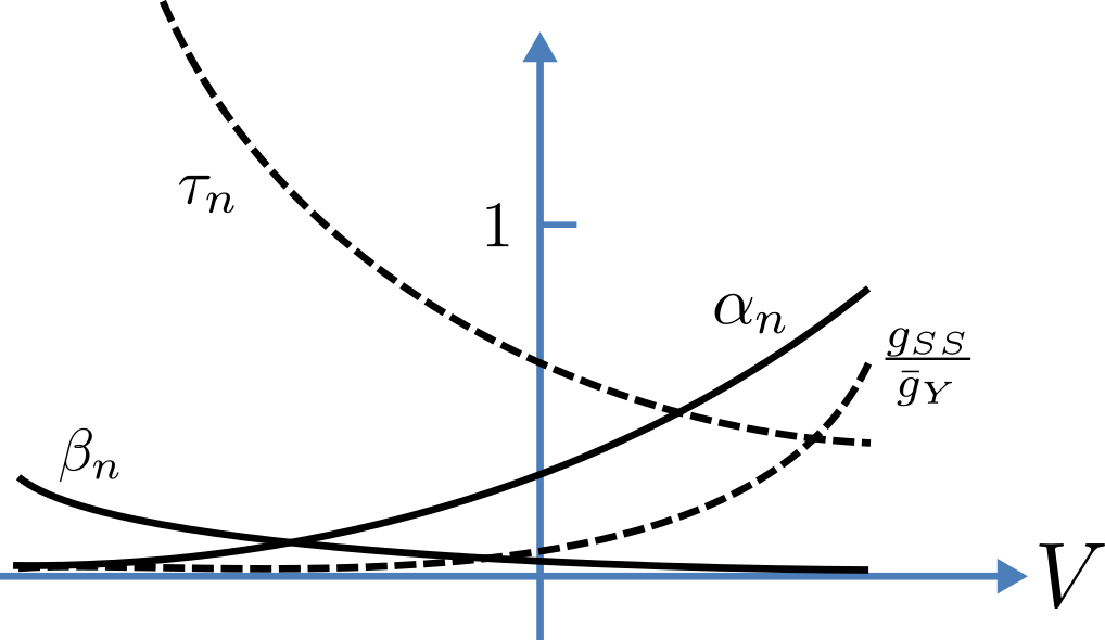
Voltage dependence of rate constants \(\alpha_n\) and \(\beta_n (\text{ms}^{-1})\), time constant \(\tau_n (\text{ms})\) and relative conductance \(\frac{g_{ss}}{\bar{g}_Y}\).

Note that under steady state conditions when \(t \rightarrow \infty\) and \(\frac{dn}{dt} \rightarrow 0\):

\[\left. \ n \right|_{t = \infty} = n_{\infty} = \frac{\alpha_{n}}{\alpha_{n} + \beta_{n}}\]

The voltage dependence of the steady state channel conductance is then:

\[g_{ss} = \left( \frac{\alpha_{n}}{\alpha_{n} + \beta_{n}} \right)^{4}.\bar{g}_{Y}\]

(see ocr_tut_volt_deps_gates). The steady state current-voltage relation for the channel is illustrated in ocr_tut_ss_cur_volt.

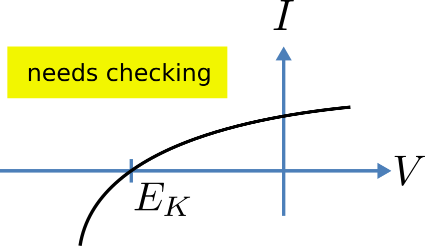
The steady-state current-voltage relation for the potassium channel.

Interpretation into a CellML model

Defining components serves two purposes: it preserves a modular structure for CellML models, and allows these component modules to be imported into other models, as demonstrated in Tutorial 6. For the potassium channel model we define components representing (i) the environment, (ii) the potassium channel conductivity, and (iii) the dynamics of the \(n\)-gate as shown in TODO.

Since certain variables (\(t\), \(V\) and \(n\)) are shared between components, we need to also define the component maps or equivalent variables as described below.

An aside: Equivalent variables

Variables are contained within components in order to make the models modular, and to enable the sharing and reuse of their different entities. But along with this containment functionality comes the need for the enclosed variables to communicate with one another across these artificial barriers. This is done by creating equivalent variable maps, wherein a variable in one component is mapped through an interface to a corresponding variable in another.

More information about how components can be nested to create a hierarchical encapsulation structure is shown in more detail in the next chapter, A model of a sodium channel and demonstrated in Tutorial 6.

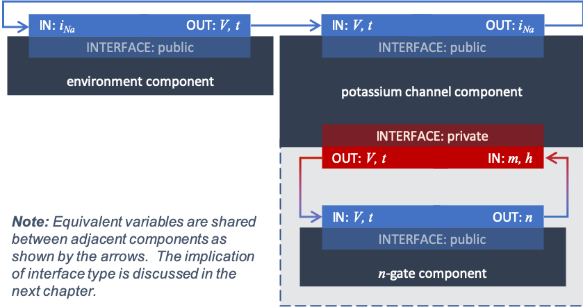
Structure of the potassium channel component with its \(n\)-gate and environment component

Simulation and results

The behaviour of the potassium channel can be simulated using the simple solver provided to run the code generated in Tutorial 6. A step change in membrane voltage between 0mV and -85mV and back gives the behaviour shown in potassium_voltage to potassium_current below. These were created using a timestep of 0.01ms to an ending time of 40ms using the simple ODE solver.

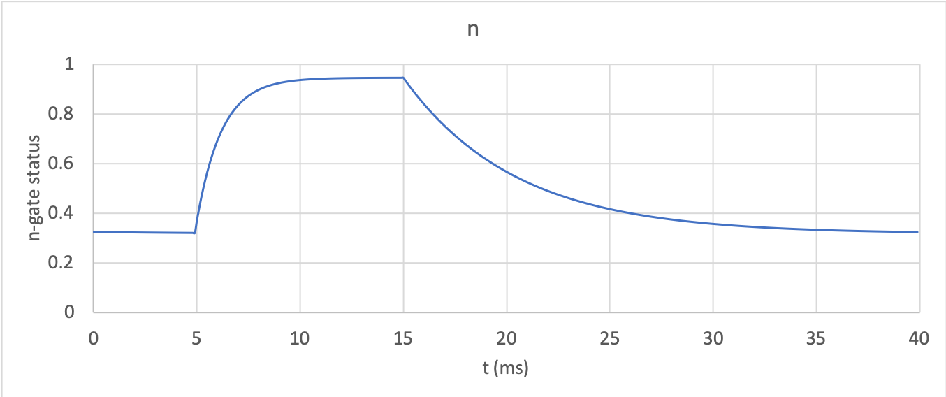
At 0mV, the steady state value of the \(n\)-gate is \(n_{\infty} = \frac{\alpha_{n}}{\alpha_{n} + \beta_{n}} =\) 0.324 and, at -85mV, \(n_{\infty} = \ \)0.945.

The voltage traces are shown in potassium_voltage. The \(n\)-gate response in potassium_ngate shows it opening beyond its initial partially open value of \(n =\)0.324 at 0mV, to plateau at an almost fully open state of \(n =\)0.945 at the Nernst potential of -85mV, before closing again as the voltage is stepped back to 0mV. Note that the opening behaviour (set by the voltage dependence of the \(\alpha_{n}\) opening rate constant) is faster than the closing behaviour (set by the voltage dependence of the \(\beta_{n}\) closing rate constant). 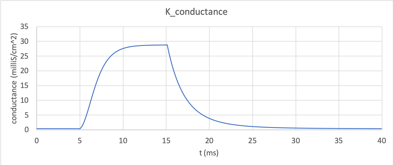The channel conductance (\(= n^{4}\bar{g}_K\)) is shown in potassium_conductance. 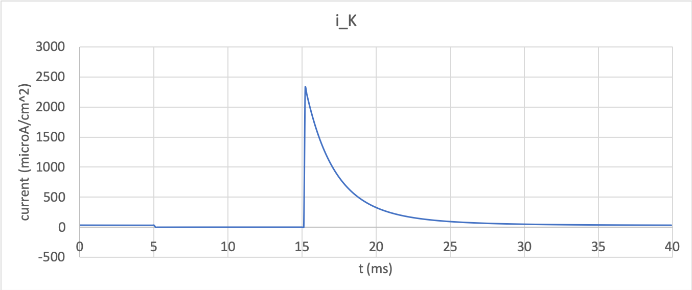Note the initial s-shaped conductance increase caused by the effect of the four gates in series \(n^{4}\) effect on conductance. Finally the channel current \(i_{K} = g_{Na}\left( V - E_{K} \right)\) is shown in potassium_current. There is no current flow during the time when the voltage is clamped at the Nernst potential (-85mV) when the gate is opening. When the voltage is stepped back to 0mV the open gates begin to close and the conductance declines, but as there is a voltage gradient it drives an outward (positive) current flow through the partially open channel. Current can only flowswhen there is a non-zero conductance and a non-zero voltage gradient. This is called the ‘tail current’.

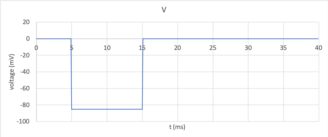
Membrane voltage clamp step from 0mv to -85mV and back.

First-order response of the n-gate to the voltage change.

Potassium channel conductance dynamics

Potassium channel current response

Note that the simulation above includes the Nernst equation with its dependence on the concentrations \(\left\lbrack K^{+} \right\rbrack_{i}\)= 90mM and \(\left\lbrack K^{+} \right\rbrack_{o}\)= 3mM. By raising the external potassium concentration to \(\left\lbrack K^{+} \right\rbrack_{o}\)= 10mM you will then see the Nernst potential increase from -85mV to -55mV and a negative (inward) current flowing during the period when the membrane voltage is clamped to -85mV. The cell is now in a ‘hyperpolarised’ state because the potential is less than the equilibrium potential.

Next steps

This potassium channel model will be used - together with a sodium channel model (in Tutorial 7) and a leakage channel model - to form the Hodgkin-Huxley neuron model (in Tutorial 8), where the membrane ion channel current flows are coupled to the equations governing current flow along the axon to generate an action potential.

The next chapter describes the theory behind the sodium channel model.

---

Footnotes

1

The original expression in the HH paper used \(\alpha_n = \frac{0.01(v+10)}{\exp\left(0.1(v+10)\right)-1}\) and \(\beta_n = 0.125\exp \left( {\frac{v}{80}} \right)\), where \(v\) is defined relative to the resting potential (\(-75\text{ mV}\)) with positive corresponding to positive inward current and \(v = -(V+75)\).